Release 2 (9.2)
Part Number A96520-01
 Home |
 Book List |
 Contents |
 Index |
 Master Index |
 Feedback |
| Oracle9i Data Warehousing Guide Release 2 (9.2) Part Number A96520-01 |
|
The following topics provide information about how to improve analytical SQL queries in a data warehouse:
Oracle has enhanced SQL's analytical processing capabilities by introducing a new family of analytic SQL functions. These analytic functions enable you to calculate:
Ranking functions include cumulative distributions, percent rank, and N-tiles. Moving window calculations allow you to find moving and cumulative aggregations, such as sums and averages. Lag/lead analysis enables direct inter-row references so you can calculate period-to-period changes. First/last analysis enables you to find the first or last value in an ordered group.
Other enhancements to SQL include the CASE expression. CASE expressions provide if-then logic useful in many situations.
To enhance performance, analytic functions can be parallelized: multiple processes can simultaneously execute all of these statements. These capabilities make calculations easier and more efficient, thereby enhancing database performance, scalability, and simplicity.
| See Also:
Oracle9i SQL Reference for further details |
Analytic functions are classified as described in Table 19-1.
To perform these operations, the analytic functions add several new elements to SQL processing. These elements build on existing SQL to allow flexible and powerful calculation expressions. With just a few exceptions, the analytic functions have these new elements. The processing flow is represented in Figure 19-1.

The essential concepts used in analytic functions are:
Query processing using analytic functions takes place in three stages. First, all joins, WHERE, GROUP BY and HAVING clauses are performed. Second, the result set is made available to the analytic functions, and all their calculations take place. Third, if the query has an ORDER BY clause at its end, the ORDER BY is processed to allow for precise output ordering. The processing order is shown in Figure 19-1.
The analytic functions allow users to divide query result sets into groups of rows called partitions. Note that the term partitions used with analytic functions is unrelated to Oracle's table partitions feature. Throughout this chapter, the term partitions refers to only the meaning related to analytic functions. Partitions are created after the groups defined with GROUP BY clauses, so they are available to any aggregate results such as sums and averages. Partition divisions may be based upon any desired columns or expressions. A query result set may be partitioned into just one partition holding all the rows, a few large partitions, or many small partitions holding just a few rows each.
For each row in a partition, you can define a sliding window of data. This window determines the range of rows used to perform the calculations for the current row. Window sizes can be based on either a physical number of rows or a logical interval such as time. The window has a starting row and an ending row. Depending on its definition, the window may move at one or both ends. For instance, a window defined for a cumulative sum function would have its starting row fixed at the first row of its partition, and its ending row would slide from the starting point all the way to the last row of the partition. In contrast, a window defined for a moving average would have both its starting and end points slide so that they maintain a constant physical or logical range.
A window can be set as large as all the rows in a partition or just a sliding window of one row within a partition. When a window is near a border, the function returns results for only the available rows, rather than warning you that the results are not what you want.
When using window functions, the current row is included during calculations, so you should only specify (n-1) when you are dealing with n items.
Each calculation performed with an analytic function is based on a current row within a partition. The current row serves as the reference point determining the start and end of the window. For instance, a centered moving average calculation could be defined with a window that holds the current row, the six preceding rows, and the following six rows. This would create a sliding window of 13 rows, as shown in Figure 19-2.

A ranking function computes the rank of a record compared to other records in the dataset based on the values of a set of measures. The types of ranking function are:
The RANK and DENSE_RANK functions allow you to rank items in a group, for example, finding the top three products sold in California last year. There are two functions that perform ranking, as shown by the following syntax:
RANK ( ) OVER ( [query_partition_clause] order_by_clause )
DENSE_RANK ( ) OVER ( [query_partition_clause] order_by_clause )
The difference between RANK and DENSE_RANK is that DENSE_RANK leaves no gaps in ranking sequence when there are ties. That is, if you were ranking a competition using DENSE_RANK and had three people tie for second place, you would say that all three were in second place and that the next person came in third. The RANK function would also give three people in second place, but the next person would be in fifth place.
The following are some relevant points about RANK:
PARTITION BY clause divide the query result set into groups within which the RANK function operates. That is, RANK gets reset whenever the group changes. In effect, the value expressions of the PARTITION BY clause define the reset boundaries.PARTITION BY clause is missing, then ranks are computed over the entire query result set.ORDER BY clause specifies the measures (<value expression>s) on which ranking is done and defines the order in which rows are sorted in each group (or partition). Once the data is sorted within each partition, ranks are given to each row starting from 1.NULLS FIRST | NULLS LAST clause indicates the position of NULLs in the ordered sequence, either first or last in the sequence. The order of the sequence would make NULLs compare either high or low with respect to non-NULL values. If the sequence were in ascending order, then NULLS FIRST implies that NULLs are smaller than all other non-NULL values and NULLS LAST implies they are larger than non-NULL values. It is the opposite for descending order. See the example in "Treatment of NULLs".NULLS FIRST | NULLS LAST clause is omitted, then the ordering of the null values depends on the ASC or DESC arguments. Null values are considered larger than any other values. If the ordering sequence is ASC, then nulls will appear last; nulls will appear first otherwise. Nulls are considered equal to other nulls and, therefore, the order in which nulls are presented is non-deterministic.The following example shows how the [ASC | DESC] option changes the ranking order.
SELECT channel_desc,
   TO_CHAR(SUM(amount_sold), '9,999,999,999') SALES$,
   RANK() OVER (ORDER BY SUM(amount_sold) ) AS default_rank,
   RANK() OVER (ORDER BY SUM(amount_sold) DESC NULLS LAST) AS custom_rank
FROM sales, products, customers, times, channels
WHERE sales.prod_id=products.prod_id AND
   sales.cust_id=customers.cust_id AND
   sales.time_id=times.time_id AND
   sales.channel_id=channels.channel_id AND
   times.calendar_month_desc IN ('2000-09', '2000-10')
    AND country_id='US'
GROUP BY channel_desc;

CHANNEL_DESC         SALES$         DEFAULT_RANK CUSTOM_RANK
-------------------- -------------- ------------ -----------
Direct Sales              5,744,263            5           1
Internet                  3,625,993            4           2
Catalog                   1,858,386            3           3
Partners                  1,500,213            2           4
Tele Sales                  604,656            1           5
While the data in this result is ordered on the measure SALES$, in general, it is not guaranteed by the RANK function that the data will be sorted on the measures. If you want the data to be sorted on SALES$ in your result, you must specify it explicitly with an ORDER BY clause, at the end of the SELECT statement.
Ranking functions need to resolve ties between values in the set. If the first expression cannot resolve ties, the second expression is used to resolve ties and so on. For example, here is a query ranking four of the sales channels over two months based on their dollar sales, breaking ties with the unit sales. (Note that the TRUNC function is used here only to create tie values for this query.)
SELECT channel_desc, calendar_month_desc,
   TO_CHAR(TRUNC(SUM(amount_sold),-6), '9,999,999,999') SALES$,
   TO_CHAR(SUM(quantity_sold), '9,999,999,999') SALES_Count,
   RANK() OVER (ORDER BY trunc(SUM(amount_sold), -6) DESC, SUM(quantity_sold)
DESC) AS col_rank
FROM sales, products, customers, times, channels
WHERE sales.prod_id=products.prod_id AND
   sales.cust_id=customers.cust_id AND
   sales.time_id=times.time_id AND
   sales.channel_id=channels.channel_id AND
   times.calendar_month_desc IN ('2000-09', '2000-10') AND
   channels.channel_desc<>'Tele Sales'
GROUP BY channel_desc, calendar_month_desc;

CHANNEL_DESC         CALENDAR SALES$         SALES_COUNT     COL_RANK
-------------------- -------- -------------- -------------- ---------
Direct Sales         2000-10      10,000,000        192,551         1
Direct Sales         2000-09       9,000,000        176,950         2
Internet             2000-10       6,000,000        123,153         3
Internet             2000-09       6,000,000        113,006         4
Catalog              2000-10       3,000,000         59,782         5
Catalog              2000-09       3,000,000         54,857         6
Partners             2000-10       2,000,000         50,773         7
Partners             2000-09       2,000,000         46,220         8
The sales_count column breaks the ties for three pairs of values.
The difference between RANK and DENSE_RANK functions is illustrated as follows:
SELECT channel_desc, calendar_month_desc,
   TO_CHAR(TRUNC(SUM(amount_sold),-6), '9,999,999,999') SALES$,
      RANK() OVER (ORDER BY trunc(SUM(amount_sold),-6) DESC)
               AS RANK,
DENSE_RANK() OVER (ORDER BY TRUNC(SUM(amount_sold),-6) DESC)
               AS DENSE_RANK
FROM sales, products, customers, times, channels
WHERE sales.prod_id=products.prod_id AND
   sales.cust_id=customers.cust_id AND
   sales.time_id=times.time_id AND
   sales.channel_id=channels.channel_id AND
   times.calendar_month_desc IN ('2000-09', '2000-10') AND
   channels.channel_desc<>'Tele Sales'
GROUP BY channel_desc, calendar_month_desc;

CHANNEL_DESC         CALENDAR SALES$              RANK DENSE_RANK
-------------------- -------- -------------- --------- ----------
Direct Sales         2000-10      10,000,000         1          1
Direct Sales         2000-09       9,000,000         2          2
Internet             2000-09       6,000,000         3          3
Internet             2000-10       6,000,000         3          3
Catalog              2000-09       3,000,000         5          4
Catalog              2000-10       3,000,000         5          4
Partners             2000-09       2,000,000         7          5
Partners             2000-10       2,000,000         7          5
Note that, in the case of DENSE_RANK, the largest rank value gives the number of distinct values in the dataset.
The RANK function can be made to operate within groups, that is, the rank gets reset whenever the group changes. This is accomplished with the PARTITION BY clause. The group expressions in the PARTITION BY subclause divide the dataset into groups within which RANK operates. For example, to rank products within each channel by their dollar sales, you say:
SELECT channel_desc, calendar_month_desc,
   TO_CHAR(SUM(amount_sold), '9,999,999,999') SALES$,
      RANK() OVER (PARTITION BY channel_desc
      ORDER BY SUM(amount_sold) DESC) AS RANK_BY_CHANNEL
FROM sales, products, customers, times, channels
WHERE sales.prod_id=products.prod_id AND
   sales.cust_id=customers.cust_id AND
   sales.time_id=times.time_id AND
   sales.channel_id=channels.channel_id AND
   times.calendar_month_desc IN ('2000-08', '2000-09', '2000-10', '2000-11') AND
   channels.channel_desc IN ('Direct Sales', 'Internet')
GROUP BY channel_desc, calendar_month_desc;
A single query block can contain more than one ranking function, each partitioning the data into different groups (that is, reset on different boundaries). The groups can be mutually exclusive. The following query ranks products based on their dollar sales within each month (rank_of_product_per_region) and within each channel (rank_of_product_total).
SELECT channel_desc, calendar_month_desc,
   TO_CHAR(SUM(amount_sold), '9,999,999,999') SALES$,
RANK() OVER (PARTITION BY calendar_month_desc
       ORDER BY SUM(amount_sold) DESC) AS RANK_WITHIN_MONTH,
 RANK() OVER (PARTITION BY channel_desc
       ORDER BY SUM(amount_sold) DESC) AS RANK_WITHIN_CHANNEL
FROM sales, products, customers, times, channels
WHERE sales.prod_id=products.prod_id AND
   sales.cust_id=customers.cust_id AND
   sales.time_id=times.time_id AND
   sales.channel_id=channels.channel_id AND
   times.calendar_month_desc IN ('2000-08', '2000-09', '2000-10', '2000-11')
    AND
   channels.channel_desc IN ('Direct Sales', 'Internet')
GROUP BY channel_desc, calendar_month_desc;
CHANNEL_DESC           CALENDAR   SALES$         RANK_WITHIN_MONTH RANK_WITHIN_CHANNEL
--------------------   --------   -------------- ----------------- -------------------
Direct Sales           2000-08         9,588,122                 1                   4
Internet               2000-08         6,084,390                 2                   4
Direct Sales           2000-09         9,652,037                 1                   3
Internet               2000-09         6,147,023                 2                   3
Direct Sales           2000-10        10,035,478                 1                   2
Internet               2000-10         6,417,697                 2                   2
Direct Sales           2000-11        12,217,068                 1                   1
Internet               2000-11         7,821,208                 2                   1
Analytic functions, RANK for example, can be reset based on the groupings provided by a CUBE, ROLLUP, or GROUPING SETS operator. It is useful to assign ranks to the groups created by CUBE, ROLLUP, and GROUPING SETS queries.
| See Also:
Chapter 18, "SQL for Aggregation in Data Warehouses" for further information about the |
A sample CUBE and ROLLUP query is the following:
SELECT channel_desc,  country_id,
   TO_CHAR(SUM(amount_sold), '9,999,999,999') SALES$,
   RANK() OVER (PARTITION BY GROUPING_ID(channel_desc, country_id)
              ORDER BY SUM(amount_sold) DESC) AS RANK_PER_GROUP
FROM sales, customers, times, channels
WHERE sales.time_id=times.time_id AND
   sales.cust_id=customers.cust_id AND
   sales.channel_id= channels.channel_id AND
   channels.channel_desc IN ('Direct Sales', 'Internet') AND
   times.calendar_month_desc='2000-09'
   AND country_id IN ('UK', 'US', 'JP')
GROUP BY CUBE( channel_desc, country_id);

CHANNEL_DESC         CO SALES$         RANK_PER_GROUP
-------------------- -- -------------- --------------
Direct Sales         US      2,835,557              1
Internet             US      1,732,240              2
Direct Sales         UK      1,378,126              3
Internet             UK        911,739              4
Direct Sales         JP         91,124              5
Internet             JP         57,232              6
Direct Sales                 4,304,807              1
Internet                     2,701,211              2
                     US      4,567,797              1
                     UK      2,289,865              2
                     JP        148,355              3
                             7,006,017              1
NULLs are treated like normal values. Also, for rank computation, a NULL value is assumed to be equal to another NULL value. Depending on the ASC | DESC options provided for measures and the NULLS FIRST | NULLS LAST clause, NULLs will either sort low or high and hence, are given ranks appropriately. The following example shows how NULLs are ranked in different cases:
SELECT calendar_year AS YEAR, calendar_quarter_number AS QTR,
            calendar_month_number AS MO, SUM(amount_sold),
RANK()  OVER (ORDER BY SUM(amount_sold)  ASC NULLS FIRST) AS NFIRST,
RANK()  OVER (ORDER BY SUM(amount_sold)  ASC NULLS LAST) AS NLASST,
RANK()  OVER (ORDER BY SUM(amount_sold)  DESC NULLS FIRST) AS NFIRST_DESC,
RANK()  OVER (ORDER BY SUM(amount_sold)  DESC NULLS LAST) AS NLAST_DESC
FROM (
       SELECT sales.time_id, sales.amount_sold, products.*, customers.*
       FROM sales, products, customers
       WHERE
         sales.prod_id=products.prod_id AND
         sales.cust_id=customers.cust_id AND
         prod_name IN ('Ruckpart Eclipse', 'Ukko Plain Gortex Boot')
         AND country_id ='UK') v, times
 WHERE v.time_id (+) =times.time_id AND
      calendar_year=1999
 GROUP BY calendar_year, calendar_quarter_number, calendar_month_number;

YEAR       QTR        MO SUM(AMOUNT_SOLD)    NFIRST    NLASST NFIRST_DESC NLAST_DESC
------------- --------- --------- ---------------- --------- --------- ----------- ----------
 1999         1         3            51820        12         8           5          1
 1999         2         6            45360        11         7           6          2
 1999         3         9            43950        10         6           7          3
 1999         3         8            41180         8         4           9          5
 1999         2         5            27431         7         3          10          6
 1999         2         4            20602         6         2          11          7
 1999         3         7            15296         5         1          12          8
 1999         1         1                          1         9           1          9
 1999         4        10                          1         9           1          9
 1999         4        11                          1         9           1          9
 1999         4        12                          1         9           1          9
If the value for two rows is NULL, the next group expression is used to resolve the tie. If they cannot be resolved even then, the next expression is used and so on till the tie is resolved or else the two rows are given the same rank. For example:
You can easily obtain top N ranks by enclosing the RANK function in a subquery and then applying a filter condition outside the subquery. For example, to obtain the top five countries in sales for a specific month, you can issue the following statement:
SELECT * FROM
  (SELECT country_id,
     TO_CHAR(SUM(amount_sold), '9,999,999,999') SALES$,
     RANK() OVER (ORDER BY SUM(amount_sold)  DESC ) AS COUNTRY_RANK
   FROM sales, products, customers, times, channels
   WHERE sales.prod_id=products.prod_id AND
     sales.cust_id=customers.cust_id AND
     sales.time_id=times.time_id AND
     sales.channel_id=channels.channel_id AND
     times.calendar_month_desc='2000-09'
   GROUP BY country_id)
WHERE COUNTRY_RANK <= 5;

CO SALES$         COUNTRY_RANK
-- -------------- ------------
US      6,517,786            1
NL      3,447,121            2
UK      3,207,243            3
DE      3,194,765            4
FR      2,125,572            5
Bottom N is similar to top N except for the ordering sequence within the rank expression. Using the previous example, you can order SUM(s_amount) ascending instead of descending.
The CUME_DIST function (defined as the inverse of percentile in some statistical books) computes the position of a specified value relative to a set of values. The order can be ascending or descending. Ascending is the default. The range of values for CUME_DIST is from greater than 0 to 1. To compute the CUME_DIST of a value x in a set S of size N, you use the formula:
CUME_DIST(x) =  number of values in S coming before and including x


in the specified order/ N
Its syntax is:
CUME_DIST ( ) OVER ( [query_partition_clause] order_by_clause )
The semantics of various options in the CUME_DIST function are similar to those in the RANK function. The default order is ascending, implying that the lowest value gets the lowest CUME_DIST (as all other values come later than this value in the order). NULLs are treated the same as they are in the RANK function. They are counted toward both the numerator and the denominator as they are treated like non-NULL values. The following example finds cumulative distribution of sales by channel within each month:
SELECT calendar_month_desc AS MONTH, channel_desc,
     TO_CHAR(SUM(amount_sold) , '9,999,999,999') SALES$ ,
     CUME_DIST() OVER ( PARTITION BY calendar_month_desc ORDER BY
         SUM(amount_sold) ) AS
     CUME_DIST_BY_CHANNEL
   FROM sales, products, customers, times, channels
   WHERE sales.prod_id=products.prod_id AND
     sales.cust_id=customers.cust_id AND
     sales.time_id=times.time_id AND
     sales.channel_id=channels.channel_id AND
     times.calendar_month_desc IN ('2000-09', '2000-07','2000-08')
   GROUP BY calendar_month_desc, channel_desc;

MONTH    CHANNEL_DESC         SALES$         CUME_DIST_BY_CHANNEL
-------- -------------------- -------------- --------------------
2000-07  Tele Sales                1,012,954                   .2
2000-07  Partners                  2,495,662                   .4
2000-07  Catalog                   2,946,709                   .6
2000-07  Internet                  6,045,609                   .8
2000-07  Direct Sales              9,563,664                    1
2000-08  Tele Sales                1,008,703                   .2
2000-08  Partners                  2,552,945                   .4
2000-08  Catalog                   3,061,381                   .6
2000-08  Internet                  6,084,390                   .8
2000-08  Direct Sales              9,588,122                    1
2000-09  Tele Sales                1,017,149                   .2
2000-09  Partners                  2,570,666                   .4
2000-09  Catalog                   3,025,309                   .6
2000-09  Internet                  6,147,023                   .8
2000-09  Direct Sales              9,652,037                    1
PERCENT_RANK is similar to CUME_DIST, but it uses rank values rather than row counts in its numerator. Therefore, it returns the percent rank of a value relative to a group of values. The function is available in many popular spreadsheets. PERCENT_RANK of a row is calculated as:
(rank of row in its partition - 1) / (number of rows in the partition - 1)
PERCENT_RANK returns values in the range zero to one. The row(s) with a rank of 1 will have a PERCENT_RANK of zero.
Its syntax is:
PERCENT_RANK ( ) OVER ( [query_partition_clause] order_by_clause )
NTILE allows easy calculation of tertiles, quartiles, deciles and other common summary statistics. This function divides an ordered partition into a specified number of groups called buckets and assigns a bucket number to each row in the partition. NTILE is a very useful calculation because it lets users divide a data set into fourths, thirds, and other groupings.
The buckets are calculated so that each bucket has exactly the same number of rows assigned to it or at most 1 row more than the others. For instance, if you have 100 rows in a partition and ask for an NTILE function with four buckets, 25 rows will be assigned a value of 1, 25 rows will have value 2, and so on. These buckets are referred to as equiheight buckets.
If the number of rows in the partition does not divide evenly (without a remainder) into the number of buckets, then the number of rows assigned for each bucket will differ by one at most. The extra rows will be distributed one for each bucket starting from the lowest bucket number. For instance, if there are 103 rows in a partition which has an NTILE(5) function, the first 21 rows will be in the first bucket, the next 21 in the second bucket, the next 21 in the third bucket, the next 20 in the fourth bucket and the final 20 in the fifth bucket.
The NTILE function has the following syntax:
NTILE ( expr ) OVER ( [query_partition_clause] order_by_clause )
In this, the N in NTILE(N) can be a constant (for example, 5) or an expression.
This function, like RANK and CUME_DIST, has a PARTITION BY clause for per group computation, an ORDER BY clause for specifying the measures and their sort order, and NULLS FIRST | NULLS LAST clause for the specific treatment of NULLs. For example,
The following is an example assigning each month's sales total into one of 4 buckets:
SELECT calendar_month_desc AS MONTH ,
     TO_CHAR(SUM(amount_sold), '9,999,999,999') SALES$,
     NTILE(4) OVER (ORDER BY SUM(amount_sold)) AS TILE4
   FROM sales, products, customers, times, channels
   WHERE sales.prod_id=products.prod_id AND
     sales.cust_id=customers.cust_id AND
     sales.time_id=times.time_id AND
     sales.channel_id=channels.channel_id AND
     times.calendar_year=1999 AND
     prod_category= 'Men'
   GROUP BY calendar_month_desc;

MONTH    SALES$             TILE4
-------- -------------- ---------
1999-10       4,373,102         1
1999-01       4,754,622         1
1999-11       5,367,943         1
1999-12       6,082,226         2
1999-07       6,161,638         2
1999-02       6,518,877         2
1999-06       6,634,401         3
1999-04       6,772,673         3
1999-08       6,954,221         3
1999-03       6,968,928         4
1999-09       7,030,524         4
1999-05       8,018,174         4
NTILE ORDER BY statements must be fully specified to yield reproducible results. Equal values can get distributed across adjacent buckets (75 is assigned to buckets 2 and 3 in the previous example) and buckets 1, 2, and 3 in the example have 3 elements - one more than the size of bucket 4. In this example, JEANS could as well be assigned to bucket 2 (instead of 3) and SWEATERS to bucket 3 (instead of 2), because there is no ordering on the p_product_key column. To ensure deterministic results, you must order on a unique key.
The ROW_NUMBER function assigns a unique number (sequentially, starting from 1, as defined by ORDER BY) to each row within the partition. It has the following syntax:
ROW_NUMBER ( ) OVER ( [query_partition_clause] order_by_clause )
SELECT channel_desc, calendar_month_desc,
   TO_CHAR(TRUNC(SUM(amount_sold), -6), '9,999,999,999') SALES$,
   ROW_NUMBER() OVER (ORDER BY TRUNC(SUM(amount_sold), -6) DESC)
     AS ROW_NUMBER
FROM sales, products, customers, times, channels
WHERE sales.prod_id=products.prod_id AND
   sales.cust_id=customers.cust_id AND
   sales.time_id=times.time_id AND
   sales.channel_id=channels.channel_id AND
   times.calendar_month_desc IN ('2000-09', '2000-10')
GROUP BY channel_desc, calendar_month_desc;

CHANNEL_DESC         CALENDAR SALES$         ROW_NUMBER
-------------------- -------- -------------- ----------
Direct Sales         2000-10      10,000,000          1
Direct Sales         2000-09       9,000,000          2
Internet             2000-09       6,000,000          3
Internet             2000-10       6,000,000          4
Catalog              2000-09       3,000,000          5
Catalog              2000-10       3,000,000          6
Partners             2000-09       2,000,000          7
Partners             2000-10       2,000,000          8
Tele Sales           2000-09       1,000,000          9
Tele Sales           2000-10       1,000,000         10
Note that there are three pairs of tie values in these results. Like NTILE, ROW_NUMBER is a non-deterministic function, so each tied value could have its row number switched. To ensure deterministic results, you must order on a unique key. Inmost cases, that will require adding a new tie breaker column to the query and using it in the ORDER BY specification.
Windowing functions can be used to compute cumulative, moving, and centered aggregates. They return a value for each row in the table, which depends on other rows in the corresponding window. These functions include moving sum, moving average, moving min/max, cumulative sum, as well as statistical functions. They can be used only in the SELECT and ORDER BY clauses of the query. Two other functions are available: FIRST_VALUE, which returns the first value in the window; and LAST_VALUE, which returns the last value in the window. These functions provide access to more than one row of a table without a self-join. The syntax of the windowing functions is:
{SUM|AVG|MAX|MIN|COUNT|STDDEV|VARIANCE|FIRST_VALUE|LAST_VALUE}
  ({value expression1 | *}) OVER
    ([PARTITION BY value expression2[,...])
      ORDER BY value expression3 [collate clause>]
                [ASC| DESC] [NULLS FIRST | NULLS LAST] [,...]
{ ROWS | RANGE }
{ BETWEEN
  { UNBOUNDED PRECEDING
  | CURRENT ROW
  | value_expr { PRECEDING | FOLLOWING }
  }
  AND
  { UNBOUNDED FOLLOWING
  | CURRENT ROW
  | value_expr { PRECEDING | FOLLOWING }
  }
| { UNBOUNDED PRECEDING
  | CURRENT ROW
  | value_expr PRECEDING
  }
}
| See Also:
Oracle9i SQL Reference for further information regarding syntax and restrictions |
Window functions' NULL semantics match the NULL semantics for SQL aggregate functions. Other semantics can be obtained by user-defined functions, or by using the DECODE or a CASE expression within the window function.
A logical offset can be specified with constants such as RANGE 10 PRECEDING, or an expression that evaluates to a constant, or by an interval specification like RANGE INTERVAL N DAY/MONTH/YEAR PRECEDING or an expression that evaluates to an interval. With logical offset, there can only be one expression in the ORDER BY expression list in the function, with type compatible to NUMERIC if offset is numeric, or DATE if an interval is specified.
The following is an example of cumulative amount_sold by customer ID by quarter in 1999:
SELECT c.cust_id, t.calendar_quarter_desc,
TO_CHAR (SUM(amount_sold), '9,999,999,999') AS Q_SALES,
TO_CHAR(SUM(SUM(amount_sold)) OVER (PARTITION BY
c.cust_id ORDER BY c.cust_id, t.calendar_quarter_desc ROWS UNBOUNDED
PRECEDING), '9,999,999,999') AS CUM_SALES
FROM sales s, times t, customers c
WHERE
s.time_id=t.time_id AND
s.cust_id=c.cust_id AND
t.calendar_year=1999 AND
c.cust_id IN (6380, 6510)
GROUP BY c.cust_id, t.calendar_quarter_desc
ORDER BY c.cust_id, t.calendar_quarter_desc;

  CUST_ID CALENDA Q_SALES        CUM_SALES
--------- ------- -------------- --------------
     6380 1999-Q1         60,621         60,621
     6380 1999-Q2         68,213        128,834
     6380 1999-Q3         75,238        204,072
     6380 1999-Q4         57,412        261,484
     6510 1999-Q1         63,030         63,030
     6510 1999-Q2         74,622        137,652
     6510 1999-Q3         69,966        207,617
     6510 1999-Q4         63,366        270,983
In this example, the analytic function SUM defines, for each row, a window that starts at the beginning of the partition (UNBOUNDED PRECEDING) and ends, by default, at the current row.
Nested SUMs are needed in this example since we are performing a SUM over a value that is itself a SUM. Nested aggregations are used very often in analytic aggregate functions.
This example of a time-based window shows, for one customer, the moving average of sales for the current month and preceding two months:
SELECT c.cust_id, t.calendar_month_desc,
TO_CHAR (SUM(amount_sold), '9,999,999,999') AS SALES ,
TO_CHAR(AVG(SUM(amount_sold))
OVER (ORDER BY c.cust_id, t.calendar_month_desc  ROWS 2 PRECEDING),
'9,999,999,999') AS MOVING_3_MONTH_AVG
FROM sales s, times t, customers c
WHERE
s.time_id=t.time_id AND
s.cust_id=c.cust_id AND
t.calendar_year=1999 AND
c.cust_id IN (6380)
GROUP BY c.cust_id, t.calendar_month_desc
ORDER BY c.cust_id, t.calendar_month_desc;

  CUST_ID CALENDAR SALES          MOVING_3_MONTH
--------- -------- -------------- --------------
     6380 1999-01          19,642         19,642
     6380 1999-02          19,324         19,483
     6380 1999-03          21,655         20,207
     6380 1999-04          27,091         22,690
     6380 1999-05          16,367         21,704
     6380 1999-06          24,755         22,738
     6380 1999-07          31,332         24,152
     6380 1999-08          22,835         26,307
     6380 1999-09          21,071         25,079
     6380 1999-10          19,279         21,062
     6380 1999-11          18,206         19,519
     6380 1999-12          19,927         19,137
Note that the first two rows for the three month moving average calculation in the output data are based on a smaller interval size than specified because the window calculation cannot reach past the data retrieved by the query. You need to consider the different window sizes found at the borders of result sets. In other words, you may need to modify the query to include exactly what you want.
Calculating windowing aggregate functions centered around the current row is straightforward. This example computes for a customer a centered moving average of the sales total for the one day preceding the current row and one day following the current row including the current row as well.
SELECT cust_id, t.time_id,
TO_CHAR (SUM(amount_sold), '9,999,999,999') AS SALES,
TO_CHAR(AVG(SUM(amount_sold)) OVER
(PARTITION BY s.cust_id ORDER BY t.time_id
RANGE BETWEEN INTERVAL '1' DAY PRECEDING AND INTERVAL '1' DAY FOLLOWING),
'9,999,999,999') AS CENTERED_3_DAY_AVG
FROM sales s, times t
WHERE
s.time_id=t.time_id AND
t.calendar_week_number IN (51) AND
calendar_year=1999 AND cust_id IN (6380, 6510)
GROUP BY cust_id, t.time_id
ORDER BY cust_id, t.time_id;

  CUST_ID TIME_ID   SALES          CENTERED_3_DAY
--------- --------- -------------- --------------
     6380 20-DEC-99          2,240          1,136
     6380 21-DEC-99             32            873
     6380 22-DEC-99            348            148
     6380 23-DEC-99             64            302
     6380 24-DEC-99            493            212
     6380 25-DEC-99             80            423
     6380 26-DEC-99            696            388
     6510 20-DEC-99            196            106
     6510 21-DEC-99             16            155
     6510 22-DEC-99            252            143
     6510 23-DEC-99            160            305
     6510 24-DEC-99            504            240
     6510 25-DEC-99             56            415
     6510 26-DEC-99            684            370
The starting and ending rows for each product's centered moving average calculation in the output data are based on just two days, since the window calculation cannot reach past the data retrieved by the query. Users need to consider the different window sizes found at the borders of result sets: the query may need to be adjusted.
The following example illustrates how window aggregate functions compute values when there are duplicates, that is, when multiple rows are returned for a single ordering value. The query retrieves the quantity sold in the US for two products during a specified time range. The query defines a moving window that runs from the date of the current row to 10 days earlier.
Note that the RANGE keyword is used to define the windowing clause of this example. This means that the window can potentially hold many rows for each value in the range. In this case, there are three rows with the duplicate ordering value of '04-NOV-98'.
SELECT time_id, s.quantity_sold,
SUM(s.quantity_sold) OVER  (ORDER BY time_id
    RANGE  BETWEEN INTERVAL '10' DAY PRECEDING AND CURRENT ROW)
AS current_group_sum
FROM  customers c, products p, sales s
WHERE  p.prod_id=s.prod_id  AND  c.cust_id=s.cust_id
   AND c.country_id='US'  AND p.prod_id IN (250, 500)
   AND s.time_id BETWEEN  '24-OCT-98' AND  '14-NOV-98'
ORDER BY TIME_ID;

TIME_ID   QUANTITY_SOLD CURRENT_GROUP_SUM  /* Source #s for row */
--------- ------------- -----------------
24-OCT-98            19                19  /*  19  */
27-OCT-98            17                36  /*  19+17  */
04-NOV-98             2                24  /*  17+(2+3+2)  */
04-NOV-98             3                24  /*  17+(2+3+2)  */
04-NOV-98             2                24  /*  17+(2+3+2)  */
14-NOV-98            12                19  /*  (2+3+2)+12 */

6 rows selected.
In the output, values within parentheses are from the rows with the tied ordering key value, 04-NOV-98.
Consider the row with the output of "04-NOV-98, 3, 24". In this case, all the other rows with TIME_ID of 04-NOV-98 (ties) are considered to belong to one group. Therefore, the CURRENT_GROUP_SUM should include this row (that is, 3) and its ties (that is, 2 and 2) in the window. It also includes any rows with dates up to 10 days earlier. In this data, that includes the row with date 27-OCT-98. Hence the result is 17+(2+3+2) = 24. The calculation of CURRENT_GROUP_SUM is identical for each of the tied rows, so the output shows three rows with the value 24.
Note that this example applies only when you use the RANGE keyword rather than the ROWS keyword. It is also important to remember that with RANGE, you can only use 1 ORDER BY expression in the analytic function's ORDER BY clause. With the ROWS keyword, you can use multiple order by expressions in the analytic function's order by clause.
There are situations where it is useful to vary the size of a window for each row, based on a specified condition. For instance, you may want to make the window larger for certain dates and smaller for others. Assume that you want to calculate the moving average of stock price over three working days. If you have an equal number of rows for each day for all working days and no non-working days are stored, then you can use a physical window function. However, if the conditions noted are not met, you can still calculate a moving average by using an expression in the window size parameters.
Expressions in a window size specification can be made in several different sources. the expression could be a reference to a column in a table, such as a time table. It could also be a function that returns the appropriate boundary for the window based on values in the current row. The following statement for a hypothetical stock price database uses a user-defined function in its RANGE clause to set window size:
SELECT t_timekey,
    AVG(stock_price)
        OVER (ORDER BY t_timekey RANGE fn(t_timekey) PRECEDING) av_price
FROM stock, time
WHERE st_timekey = t_timekey
ORDER BY t_timekey;
In this statement, t_timekey is a date field. Here, fn could be a PL/SQL function with the following specification:
fn(t_timekey) returns
t_timekey is Monday, TuesdayNote that, when window is specified using a number in a window function with ORDER BY on a date column, then it is converted to mean the number of days. You could have also used the interval literal conversion function, as NUMTODSINTERVAL(fn(t_timekey), 'DAY') instead of just fn(t_timekey) to mean the same thing. You can also write a PL/SQL function that returns an INTERVAL datatype value.
For windows expressed in rows, the ordering expressions should be unique to produce deterministic results. For example, the following query is not deterministic because time_id is not unique in this result set.
SELECT t.time_id,
TO_CHAR(amount_sold, '9,999,999,999') AS INDIV_SALE,
TO_CHAR(SUM(amount_sold) OVER
(PARTITION BY t.time_id ORDER BY t.time_id
ROWS UNBOUNDED PRECEDING), '9,999,999,999') AS CUM_SALES
FROM sales s, times t, customers c
WHERE
s.time_id=t.time_id AND
s.cust_id=c.cust_id AND
t.time_id IN (TO_DATE('11-DEC-1999'), TO_DATE('12-DEC-1999') )
  AND
c.cust_id BETWEEN 6500 AND 6600
ORDER BY t.time_id;

TIME_ID   INDIV_SALE     CUM_SALES
--------- -------------- --------------
11-DEC-99          1,036          1,036
11-DEC-99          1,932          2,968
11-DEC-99            588          3,556
12-DEC-99            504            504
12-DEC-99            429            933
12-DEC-99          1,160          2,093
The statement could also yield the following:
TIME_ID   INDIV_SALE     CUM_SALES
--------- -------------- --------------
11-DEC-99          1,932          2,968
11-DEC-99            588          3,556
11-DEC-99          1,036          1,036
12-DEC-99            504            504
12-DEC-99          1,160          2,093
12-DEC-99            429            933
One way to handle this problem would be to add the prod_id column to the result set and order on both time_id and prod_id.
The FIRST_VALUE and LAST_VALUE functions allow you to select the first and last rows from a window. These rows are especially valuable because they are often used as the baselines in calculations. For instance, with a partition holding sales data ordered by day, you might ask "How much was each day's sales compared to the first sales day (FIRST_VALUE) of the period?" Or you might wish to know, for a set of rows in increasing sales order, "What was the percentage size of each sale in the region compared to the largest sale (LAST_VALUE) in the region?"
After a query has been processed, aggregate values like the number of resulting rows or an average value in a column can be easily computed within a partition and made available to other reporting functions. Reporting aggregate functions return the same aggregate value for every row in a partition. Their behavior with respect to NULLs is the same as the SQL aggregate functions. The syntax is:
{SUM | AVG | MAX | MIN | COUNT | STDDEV | VARIANCE}
   ([ALL | DISTINCT] {value expression1 | *})
       OVER ([PARTITION BY value expression2[,...]])
In addition, the following conditions apply:
COUNT(*)DISTINCT is supported only if corresponding aggregate functions allow itvalue expression1 and value expression2 can be any valid expression involving column references or aggregates.PARTITION BY clause defines the groups on which the windowing functions would be computed. If the PARTITION BY clause is absent, then the function is computed over the whole query result set.Reporting functions can appear only in the SELECT clause or the ORDER BY clause. The major benefit of reporting functions is their ability to do multiple passes of data in a single query block and speed up query performance. Queries such as "Count the number of salesmen with sales more than 10% of city sales" do not require joins between separate query blocks.
For example, consider the question "For each product category, find the region in which it had maximum sales". The equivalent SQL query using the MAX reporting aggregate function would be:
SELECT prod_category, country_region, sales FROM
(SELECT substr(p.prod_category,1,8), co.country_region, SUM(amount_sold)
  AS sales,
MAX(SUM(amount_sold)) OVER (partition BY prod_category) AS MAX_REG_SALES
FROM sales s, customers c, countries co, products p
WHERE s.cust_id=c.cust_id AND
c.country_id=co.country_id AND
s.prod_id=p.prod_id AND
s.time_id=to_DATE('11-OCT-2000')
GROUP BY prod_category, country_region)
WHERE sales=MAX_REG_SALES;
The inner query with the reporting aggregate function MAX(SUM(amount_sold)) returns:
SUBSTR(P COUNTRY_REGION           SALES MAX_REG_SALES
-------- -------------------- --------- -------------
Boys     Africa                     594         41974
Boys     Americas                 20353         41974
Boys     Asia                      2258         41974
Boys     Europe                   41974         41974
Boys     Oceania                   1402         41974
Girls    Americas                 13869         52963
Girls    Asia                      1657         52963
Girls    Europe                   52963         52963
Girls    Middle East                303         52963
Girls    Oceania                    380         52963
Men      Africa                    1705        123253
Men      Americas                 69304        123253
Men      Asia                      6153        123253
Men      Europe                  123253        123253
Men      Oceania                   2646        123253
Women    Africa                    4037        255109
Women    Americas                145501        255109
Women    Asia                     20394        255109
Women    Europe                  255109        255109
Women    Middle East                350        255109
Women    Oceania                  17408        255109
The full query results are:
PROD_CATEGORY      COUNTRY_REGION    SALES
-------------      --------------    ------
Boys               Europe             41974
Girls              Europe             52963
Men                Europe            123253
Women              Europe            255109
Reporting aggregates combined with nested queries enable you to answer complex queries efficiently. For instance, what if we want to know the best selling products in our most significant product subcategories? We have 4 product categories which contain a total of 37 product subcategories, and there are 10,000 unique products. Here is a query which finds the 5 top-selling products for each product subcategory that contributes more than 20% of the sales within its product category.
SELECT SUBSTR(prod_category,1,8) AS CATEG, prod_subcategory, prod_id, SALES FROM
  (SELECT p.prod_category, p.prod_subcategory, p.prod_id,
      SUM(amount_sold) as SALES,
      SUM(SUM(amount_sold)) OVER (PARTITION BY p.prod_category) AS CAT_SALES,
      AUM(SUM(amount_sold)) OVER
         (PARTITION BY p.prod_subcategory) AS SUBCAT_SALES,
      RANK() OVER  (PARTITION BY p.prod_subcategory
         ORDER BY SUM(amount_sold) ) AS RANK_IN_LINE
     FROM sales s, customers c, countries co, products p
     WHERE s.cust_id=c.cust_id AND
        c.country_id=co.country_id AND  s.prod_id=p.prod_id AND
        s.time_id=to_DATE('11-OCT-2000')
     GROUP BY p.prod_category, p.prod_subcategory, p.prod_id
     ORDER BY prod_category, prod_subcategory)
  WHERE SUBCAT_SALES>0.2*CAT_SALES AND RANK_IN_LINE<=5;
The RATIO_TO_REPORT function computes the ratio of a value to the sum of a set of values. If the expression value expression evaluates to NULL, RATIO_TO_REPORT also evaluates to NULL, but it is treated as zero for computing the sum of values for the denominator. Its syntax is:
RATIO_TO_REPORT ( expr ) OVER ( [query_partition_clause] )
In this, the following applies:
expr can be any valid expression involving column references or aggregates.PARTITION BY clause defines the groups on which the RATIO_TO_REPORT function is to be computed. If the PARTITION BY clause is absent, then the function is computed over the whole query result set.To calculate RATIO_TO_REPORT of sales per channel, you might use the following syntax:
SELECT ch.channel_desc,
    TO_CHAR(SUM(amount_sold),'9,999,999') as SALES,
    TO_CHAR(SUM(SUM(amount_sold)) OVER (), '9,999,999')
        AS TOTAL_SALES,
    TO_CHAR(RATIO_TO_REPORT(SUM(amount_sold)) OVER (), '9.999')
        AS RATIO_TO_REPORT
     FROM sales s, channels ch
     WHERE s.channel_id=ch.channel_id  AND
        s.time_id=to_DATE('11-OCT-2000')
     GROUP BY ch.channel_desc;

CHANNEL_DESC         SALES      TOTAL_SALE RATIO_
-------------------- ---------- ---------- ------
Catalog                 111,103    781,613   .142
Direct Sales            335,409    781,613   .429
Internet                212,314    781,613   .272
Partners                 91,352    781,613   .117
Tele Sales               31,435    781,613   .040
The LAG and LEAD functions are useful for comparing values when the relative positions of rows can be known reliably. They work by specifying the count of rows which separate the target row from the current row. Since the functions provide access to more than one row of a table at the same time without a self-join, they can enhance processing speed. The LAG function provides access to a row at a given offset prior to the current position, and the LEAD function provides access to a row at a given offset after the current position.
These functions have the following syntax:
{LAG | LEAD} ( value_expr [, offset] [, default] )
   OVER ( [query_partition_clause] order_by_clause )
offset is an optional parameter and defaults to 1. default is an optional parameter and is the value returned if offset falls outside the bounds of the table or partition.
SELECT  time_id, TO_CHAR(SUM(amount_sold),'9,999,999') AS SALES,
TO_CHAR(LAG(SUM(amount_sold),1) OVER (ORDER BY time_id),'9,999,999') AS LAG1,
TO_CHAR(LEAD(SUM(amount_sold),1) OVER (ORDER BY time_id),'9,999,999') AS LEAD1
FROM sales
WHERE
time_id>=TO_DATE('10-OCT-2000') AND
time_id<=TO_DATE('14-OCT-2000')
GROUP BY time_id;

TIME_ID   SALES      LAG1       LEAD1
--------- ---------- ---------- ----------
10-OCT-00    773,921               781,613
11-OCT-00    781,613    773,921    744,351
12-OCT-00    744,351    781,613    757,356
13-OCT-00    757,356    744,351    791,960
14-OCT-00    791,960    757,356
The FIRST/LAST aggregate functions allow you to return the result of an aggregate applied over a set of rows that rank as the first or last with respect to a given order specification. FIRST/LAST lets you order on column A but return an result of an aggregate applied on column B. This is valuable because it avoids the need for a self-join or subquery, thus improving performance. These functions begin with a tiebreaker function, which is a regular aggregate function (MIN, MAX, SUM, AVG, COUNT, VARIANCE, STDDEV) that produces the return value. The tiebreaker function is performed on the set rows (1 or more rows) that rank as first or last respect to the order specification to return a single value.
To specify the ordering used within each group, the FIRST/LAST functions add a new clause starting with the word KEEP.
These functions have the following syntax:
aggregate_function KEEP
( DENSE_RANK LAST ORDER BY
  expr [ DESC | ASC ] [NULLS { FIRST | LAST }]
  [, expr [ DESC | ASC ] [NULLS { FIRST | LAST }]]...
)
[OVER query_partitioning_clause]
Note that the ORDER BY clause can take multiple expressions.
You can use the FIRST/LAST family of aggregates as regular aggregate functions.
The following query lets us compare minimum price and list price of our products. For each product subcategory within the Men's clothing category, it returns the following:
SELECT prod_subcategory, MIN(prod_list_price)KEEP (DENSE_RANK FIRST ORDER BY (prod_min_price))AS LP_OF_LO_MINP,MIN(prod_min_price) AS LO_MINP,MAX(prod_list_price) KEEP (DENSE_RANK LAST ORDER BY (prod_min_price))AS LP_OF_HI_MINP,MAX(prod_min_price) AS HI_MINPFROM productsWHERE prod_category='Men'GROUP BY prod_subcategory;PROD_SUBCATEGORY LP_OF_LO_MINP LO_MINP LP_OF_HI_MINP HI_MINP---------------- ------------- ------- ------------- -------Casual Shirts - Men 39.9 16.92 88 59.4Dress Shirts - Men 42.5 17.34 59.9 41.51Jeans - Men 38 17.33 69.9 62.28Outerwear - Men 44.9 19.76 495 334.12Shorts - Men 34.9 15.36 195 103.54Sportcoats - Men 195 96.53 595 390.92Sweaters - Men 29.9 14.59 140 97.02Trousers - Men 38 15.5 135 120.29Underwear And Socks - Men 10.9 4.45 39.5 27.02
A query like this can be useful for understanding the sales patterns of your different channels. For instance, the result set here highlights that Telesales sell relatively small volumes.
You can also use the FIRST/LAST family of aggregates as reporting aggregate functions. An example is calculating which months had the greatest and least increase in head count throughout the year. The syntax for these functions is similar to the syntax for any other reporting aggregate.
Consider the example in Example 19-11 for FIRST/LAST. What if we wanted to find the list prices of individual products and compare them to the list prices of the products in their subcategory that had the highest and lowest minimum prices?
The following query lets us find that information for the Sportcoats - Men subcategory by using FIRST/LAST as reporting aggregates. Because there are over 100 products in this subcategory, we show only the first few rows of results.
SELECT prod_id, prod_list_price,
MIN(prod_list_price) KEEP (DENSE_RANK FIRST ORDER BY (prod_min_price))
  OVER(PARTITION BY (prod_subcategory)) AS LP_OF_LO_MINP,
MAX(prod_list_price) KEEP (DENSE_RANK LAST ORDER BY (prod_min_price))
  OVER(PARTITION BY (prod_subcategory)) AS  LP_OF_HI_MINP
FROM products
WHERE prod_subcategory='Sportcoats - Men';

PROD_ID      PROD_LIST_PRICE       LP_OF_LO_MINP     LP_OF_HI_MINP
-------      ---------------       -------------     -------------
    730                  365                 195               595
   1165                  365                 195               595
   1560                  595                 195               595
   2655                  195                 195               595
   2660                  195                 195               595
   3840                  275                 195               595
   3865                  275                 195               595
   4035                319.9                 195               595
   4075                  395                 195               595
   4245                  195                 195               595
   4790                  365                 195               595
   4800                  365                 195               595
   5560                  425                 195               595
   5575                  425                 195               595
   5625                  595                 195               595
   7915                  275                 195               595
....
Using the FIRST and LAST functions as reporting aggregates makes it easy to include the results in calculations such "Salary as a percent of the highest salary."
The regression functions support the fitting of an ordinary-least-squares regression line to a set of number pairs. You can use them as both aggregate functions or windowing or reporting functions.
The functions are:
Oracle applies the function to the set of (e1, e2) pairs after eliminating all pairs for which either of e1 or e2 is null. e1 is interpreted as a value of the dependent variable (a "y value"), and e2 is interpreted as a value of the independent variable (an "x value"). Both expressions must be numbers.
The regression functions are all computed simultaneously during a single pass through the data. They are frequently combined with the COVAR_POP, COVAR_SAMP, and CORR functions.
| See Also:
Oracle9i SQL Reference for further information regarding syntax and semantics |
REGR_COUNT returns the number of non-null number pairs used to fit the regression line. If applied to an empty set (or if there are no (e1, e2) pairs where neither of e1 or e2 is null), the function returns 0.
REGR_AVGY and REGR_AVGX compute the averages of the dependent variable and the independent variable of the regression line, respectively. REGR_AVGY computes the average of its first argument (e1) after eliminating (e1, e2) pairs where either of e1 or e2 is null. Similarly, REGR_AVGX computes the average of its second argument (e2) after null elimination. Both functions return NULL if applied to an empty set.
The REGR_SLOPE function computes the slope of the regression line fitted to non-null (e1, e2) pairs.
The REGR_INTERCEPT function computes the y-intercept of the regression line. REGR_INTERCEPT returns NULL whenever slope or the regression averages are NULL.
The REGR_R2 function computes the coefficient of determination (usually called "R-squared" or "goodness of fit") for the regression line.
REGR_R2 returns values between 0 and 1 when the regression line is defined (slope of the line is not null), and it returns NULL otherwise. The closer the value is to 1, the better the regression line fits the data.
REGR_SXX, REGR_SYY and REGR_SXY functions are used in computing various diagnostic statistics for regression analysis. After eliminating (e1, e2) pairs where either of e1 or e2 is null, these functions make the following computations:
REGR_SXX:    REGR_COUNT(e1,e2) * VAR_POP(e2)

REGR_SYY:    REGR_COUNT(e1,e2) * VAR_POP(e1)

REGR_SXY:    REGR_COUNT(e1,e2) * COVAR_POP(e1, e2)
Some common diagnostic statistics that accompany linear regression analysis are given in Table 19-2, "Common Diagnostic Statistics and Their Expressions". Note that Oracle's new functions allow you to calculate all of these.
In this example, we compute an ordinary-least-squares regression line that expresses the quantity sold of a product as a linear function of the product's list price. The calculations are grouped by sales channel. The values SLOPE, INTCPT, RSQR are slope, intercept, and coefficient of determination of the regression line, respectively. The (integer) value COUNT is the number of products in each channel for whom both quantity sold and list price data are available.
SELECT s.channel_id,
REGR_SLOPE(s.quantity_sold, p.prod_list_price) SLOPE,
REGR_INTERCEPT(s.quantity_sold, p.prod_list_price) INTCPT,
REGR_R2(s.quantity_sold, p.prod_list_price) RSQR,
REGR_COUNT(s.quantity_sold, p.prod_list_price) COUNT,
REGR_AVGX(s.quantity_sold, p.prod_list_price) AVGLISTP,
REGR_AVGY(s.quantity_sold, p.prod_list_price) AVGQSOLD
FROM sales s, products p
WHERE s.prod_id=p.prod_id
  AND p.prod_category='Men' AND s.time_id=to_DATE('10-OCT-2000')
GROUP BY s.channel_id;

C     SLOPE    INTCPT      RSQR     COUNT  AVGLISTP  AVGQSOLD
- --------- --------- --------- --------- --------- ---------
C -.0683687 16.627808 .05134258        20    65.495     12.15
I  .0197103 14.811392 .00163149        46 51.480435 15.826087
P -.0124736 12.854546 .01703979        30     81.87 11.833333
S .00615589 13.991924 .00089844        83 69.813253 14.421687
T -.0041131 5.2271721 .00813224        27 82.244444 4.8888889
Using the CUME_DIST function, you can find the cumulative distribution (percentile) of a set of values. However, the inverse operation (finding what value computes to a certain percentile) is neither easy to do nor efficiently computed. To overcome this difficulty, Oracle introduced the PERCENTILE_CONT and PERCENTILE_DISC functions. These can be used both as window reporting functions as well as normal aggregate functions.
These functions need a sort specification and a parameter that takes a percentile value between 0 and 1. The sort specification is handled by using an ORDER BY clause with one expression. When used as a normal aggregate function, it returns a single value for each ordered set.
PERCENTILE_CONT, which is a continuous function computed by interpolation, and PERCENTILE_DISC, which is a step function that assumes discrete values. Like other aggregates, PERCENTILE_CONT and PERCENTILE_DISC operate on a group of rows in a grouped query, but with the following differences:
ORDER BY clause with a single expression. Multiple expressions are not allowed.[PERCENTILE_CONT | PERCENTILE_DISC]( constant expression ) WITHIN GROUP ( ORDER BY single order by expression [ASC|DESC] [NULLS FIRST| NULLS LAST])
We use the following query to return the 17 rows of data used in the examples of this section:
SELECT cust_id, cust_credit_limit, CUME_DIST()
   OVER (ORDER BY cust_credit_limit) AS CUME_DIST
FROM customers
WHERE cust_city='Marshal';

CUST_ID   CUST_CREDIT_LIMIT CUME_DIST
--------- ----------------- ---------
   171630              1500 .23529412
   346070              1500 .23529412
   420830              1500 .23529412
   383450              1500 .23529412
   165400              3000 .35294118
   227700              3000 .35294118
    28340              5000 .52941176
   215240              5000 .52941176
   364760              5000 .52941176
   184090              7000 .70588235
   370990              7000 .70588235
   408370              7000 .70588235
   121790              9000 .76470588
    22110             11000 .94117647
   246390             11000 .94117647
    40800             11000 .94117647
   464440             15000         1
PERCENTILE_DISC(x) is computed by scanning up the CUME_DIST values in each group till you find the first one greater than or equal to x, where x is the specified percentile value. For the example query where PERCENTILE_DISC(0.5), the result is 5,000, as the following illustrates:
SELECT PERCENTILE_DISC(0.5) WITHIN GROUP
  (ORDER BY cust_credit_limit) AS perc_disc,
   PERCENTILE_CONT(0.5) WITHIN GROUP
  (ORDER BY cust_credit_limit) AS perc_cont
 FROM customers WHERE cust_city='Marshal';

PERC_DISC   PERC_CONT
---------   ---------
     5000        5000
The result of PERCENTILE_CONT is computed by linear interpolation between rows after ordering them. To compute PERCENTILE_CONT(x), we first compute the row number = RN= (1+x*(n-1)), where n is the number of rows in the group and x is the specified percentile value. The final result of the aggregate function is computed by linear interpolation between the values from rows at row numbers CRN = CEIL(RN) and FRN = FLOOR(RN).
The final result will be: PERCENTILE_CONT(X) = if (CRN = FRN = RN), then (value of expression from row at RN) else (CRN - RN) * (value of expression for row at FRN) + (RN -FRN) * (value of expression for row at CRN).
Consider the previous example query, where we compute PERCENTILE_CONT(0.5). Here n is 17. The row number RN = (1 + 0.5*(n-1))= 9 for both groups. Putting this into the formula, (FRN=CRN=9), we return the value from row 9 as the result.
Another example is, if you want to compute PERCENTILE_CONT(0.66). The computed row number RN=(1 + 0.66*(n-1))= (1 + 0.66*16)= 11.67. PERCENTILE_CONT(0.66) = (12-11.67)*(value of row 11)+(11.67-11)*(value of row 12). These results are:
SELECT PERCENTILE_DISC(0.66) WITHIN GROUP
  (ORDER BY cust_credit_limit) AS perc_disc,
   PERCENTILE_CONT(0.66) WITHIN GROUP
  (ORDER BY cust_credit_limit) AS perc_cont
 FROM customers WHERE cust_city='Marshal';

PERC_DISC   PERC_CONT
---------   ---------
     7000        7000
Inverse percentile aggregate functions can appear in the HAVING clause of a query like other existing aggregate functions.
You can also use the aggregate functions PERCENTILE_CONT, PERCENTILE_DISC as reporting aggregate functions. When used as reporting aggregate functions, the syntax is similar to those of other reporting aggregates.
[PERCENTILE_CONT | PERCENTILE_DISC](constant expression)
WITHIN GROUP ( ORDER BY single order by expression
[ASC|DESC] [NULLS FIRST| NULLS LAST])
OVER ( [PARTITION BY value expression [,...]] )
This query computes the same thing (median credit limit for customers in this result set, but reports the result for every row in the result set, as shown in the following output:
SELECT cust_id, cust_credit_limit,
   PERCENTILE_DISC(0.5) WITHIN GROUP
     (ORDER BY cust_credit_limit) OVER () AS perc_disc,
   PERCENTILE_CONT(0.5) WITHIN GROUP
     (ORDER BY cust_credit_limit) OVER () AS perc_cont
 FROM customers WHERE cust_city='Marshal';

CUST_ID   CUST_CREDIT_LIMIT PERC_DISC PERC_CONT
--------- ----------------- --------- ---------
   171630              1500      5000      5000
   346070              1500      5000      5000
   420830              1500      5000      5000
   383450              1500      5000      5000
   165400              3000      5000      5000
   227700              3000      5000      5000
    28340              5000      5000      5000
   215240              5000      5000      5000
   364760              5000      5000      5000
   184090              7000      5000      5000
   370990              7000      5000      5000
   408370              7000      5000      5000
   121790              9000      5000      5000
    22110             11000      5000      5000
   246390             11000      5000      5000
    40800             11000      5000      5000
   464440             15000      5000      5000
For PERCENTILE_DISC, the expression in the ORDER BY clause can be of any data type that you can sort (numeric, string, date, and so on). However, the expression in the ORDER BY clause must be a numeric or datetime type (including intervals) because linear interpolation is used to evaluate PERCENTILE_CONT. If the expression is of type DATE, the interpolated result is rounded to the smallest unit for the type. For a DATE type, the interpolated value will be rounded to the nearest second, for interval types to the nearest second (INTERVAL DAY TO SECOND) or to the month(INTERVAL YEAR TO MONTH).
Like other aggregates, the inverse percentile functions ignore NULLs in evaluating the result. For example, when you want to find the median value in a set, Oracle ignores the NULLs and finds the median among the non-null values. You can use the NULLS FIRST/NULLS LAST option in the ORDER BY clause, but they will be ignored as NULLs are ignored.
These functions provide functionality useful for what-if analysis. As an example, what would be the rank of a row, if the row was hypothetically inserted into a set of other rows?
This family of aggregates takes one or more arguments of a hypothetical row and an ordered group of rows, returning the RANK, DENSE_RANK, PERCENT_RANK or CUME_DIST of the row as if it was hypothetically inserted into the group.
[RANK | DENSE_RANK | PERCENT_RANK | CUME_DIST]( constant expression [, ...] )
WITHIN GROUP ( ORDER BY order by expression [ASC|DESC] [NULLS FIRST|NULLS
LAST][, ...] )
Here, constant expression refers to an expression that evaluates to a constant, and there may be more than one such expressions that are passed as arguments to the function. The ORDER BY clause can contain one or more expressions that define the sorting order on which the ranking will be based. ASC, DESC, NULLS FIRST, NULLS LAST options will be available for each expression in the ORDER BY.
Using the list price data from the products table used throughout this section, you can calculate the RANK, PERCENT_RANK and CUME_DIST for a hypothetical sweater with a price of $50 for how it fits within each of the sweater subcategories. The query and results are:
SELECT prod_subcategory,
 RANK(50) WITHIN GROUP  (ORDER BY prod_list_price DESC) AS HRANK,
  TO_CHAR(PERCENT_RANK(50) WITHIN GROUP
      (ORDER BY prod_list_price),'9.999') AS HPERC_RANK,
  TO_CHAR(CUME_DIST (50) WITHIN GROUP
      (ORDER BY prod_list_price),'9.999') AS HCUME_DIST
FROM products
WHERE prod_subcategory LIKE 'Sweater%'
GROUP BY prod_subcategory;

PROD_SUBCATEGORY               HRANK   HPERC_RANK   HCUME_DIST
----------------               -----   ----------   ----------
Sweaters - Boys                   16         .911         .912
Sweaters - Girls                   1        1.000        1.000
Sweaters - Men                   240         .351         .352
Sweaters - Women                  21         .783         .785
Unlike the inverse percentile aggregates, the ORDER BY clause in the sort specification for hypothetical rank and distribution functions may take multiple expressions. The number of arguments and the expressions in the ORDER BY clause should be the same and the arguments must be constant expressions of the same or compatible type to the corresponding ORDER BY expression. The following is an example using two arguments in several hypothetical ranking functions.
SELECT prod_subcategory,
 RANK(45,30) WITHIN GROUP  (ORDER BY prod_list_price DESC,prod_min_price) AS
HRANK,
  TO_CHAR(PERCENT_RANK(45,30) WITHIN GROUP
      (ORDER BY prod_list_price, prod_min_price),'9.999') AS HPERC_RANK,
  TO_CHAR(CUME_DIST (45,30) WITHIN GROUP
      (ORDER BY prod_list_price, prod_min_price),'9.999') AS HCUME_DIST
FROM products
WHERE prod_subcategory
  LIKE 'Sweater%'
GROUP BY prod_subcategory;

PROD_SUBCATEGORY              HRANK     HPERC_RANK  HCUME_DIST
----------------              -----     ----------  ----------
Sweaters - Boys                  21           .858        .859
Sweaters - Girls                  1          1.000       1.000
Sweaters - Men                  340           .079        .081
Sweaters - Women                 72           .228        .237
These functions can appear in the HAVING clause of a query just like other aggregate functions. They cannot be used as either reporting aggregate functions or windowing aggregate functions.
For a given expression, the WIDTH_BUCKET function returns the bucket number that the result of this expression will be assigned after it is evaluated. You can generate equiwidth histograms with this function. Equiwidth histograms divide data sets into buckets whose interval size (highest value to lowest value) is equal. The number of rows held by each bucket will vary. A related function, NTILE, creates equiheight buckets.
Equiwidth histograms can be generated only for numeric, date or datetime types. So the first three parameters should be all numeric expressions or all date expressions. Other types of expressions are not allowed. If the first parameter is NULL, the result is NULL. If the second or the third parameter is NULL, an error message is returned, as a NULL value cannot denote any end point (or any point) for a range in a date or numeric value dimension. The last parameter (number of buckets) should be a numeric expression that evaluates to a positive integer value; 0, NULL, or a negative value will result in an error.
Buckets are numbered from 0 to (n+1). Bucket 0 holds the count of values less than the minimum. Bucket(n+1) holds the count of values greater than or equal to the maximum specified value.
The WIDTH_BUCKET takes four expressions as parameters. The first parameter is the expression that the equiwidth histogram is for. The second and third parameters are expressions that denote the end points of the acceptable range for the first parameter. The fourth parameter denotes the number of buckets.
WIDTH_BUCKET(expression, minval expression, maxval expression, num buckets)
Consider the following data from table customers, that shows the credit limits of 17 customers. This data is gathered in the query shown in Example 19-15.
CUST_ID  CUST_CREDIT_LIMIT
-------- -----------------
   22110             11000
   28340              5000
   40800             11000
  121790              9000
  165400              3000
  171630              1500
  184090              7000
  215240              5000
  227700              3000
  246390             11000
  346070              1500
  364760              5000
  370990              7000
  383450              1500
  408370              7000
  420830              1500
  464440             15000
In the table customers, the column cust_credit_limit contains values between 1500 and 15000, and we can assign the values to four equiwidth buckets, numbered from 1 to 4, by using WIDTH_BUCKET (cust_credit_limit, 0, 20000, 4). Ideally each bucket is a closed-open interval of the real number line, for example, bucket number 2 is assigned to scores between 5000.0000 and 9999.9999..., sometimes denoted [5000, 10000) to indicate that 5,000 is included in the interval and 10,000 is excluded. To accommodate values outside the range [0, 20,000), values less than 0 are assigned to a designated underflow bucket which is numbered 0, and values greater than or equal to 20,000 are assigned to a designated overflow bucket which is numbered 5 (num buckets + 1 in general). See Figure 19-3 for a graphical illustration of how the buckets are assigned.
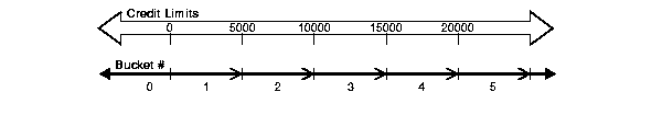
You can specify the bounds in the reverse order, for example, WIDTH_BUCKET (cust_credit_limit, 20000, 0, 4). When the bounds are reversed, the buckets will be open-closed intervals. In this example, bucket number 1 is (15000,20000], bucket number 2 is (10000,15000], and bucket number 4, is (0,5000]. The overflow bucket will be numbered 0 (20000, +infinity), and the underflow bucket will be numbered 5 (-infinity, 0].
It is an error if the bucket count parameter is 0 or negative.
The following query shows the bucket numbers for the credit limits in the customers table for both cases where the boundaries are specified in regular or reverse order. We use a range of 0 to 20,000.
SELECT cust_id, cust_credit_limit,
  WIDTH_BUCKET(cust_credit_limit,0,20000,4) AS WIDTH_BUCKET_UP,
  WIDTH_BUCKET(cust_credit_limit,20000, 0, 4) AS WIDTH_BUCKET_DOWN
FROM customers WHERE cust_city = 'Marshal';

  CUST_ID CUST_CREDIT_LIMIT WIDTH_BUCKET_UP WIDTH_BUCKET_DOWN
  ------- ----------------- --------------- -----------------
    22110             11000               3                 2
    28340              5000               2                 4
    40800             11000               3                 2
   121790              9000               2                 3
   165400              3000               1                 4
   171630              1500               1                 4
   184090              7000               2                 3
   215240              5000               2                 4
   227700              3000               1                 4
   246390             11000               3                 2
   346070              1500               1                 4
   364760              5000               2                 4
   370990              7000               2                 3
   383450              1500               1                 4
   408370              7000               2                 3
   420830              1500               1                 4
   464440             15000               4                 2
Oracle offers a facility for creating your own functions, called user-defined aggregate functions. These functions are written in programming languages such as PL/SQL, Java, and C, and can be used as analytic functions or aggregates in materialized views.
| See Also:
Oracle9i Data Cartridge Developer's Guide for further information regarding syntax and restrictions |
The advantages of these functions are:
As a simple example of a user-defined aggregate function, consider the skew statistic. This calculation measures if a data set has a lopsided distribution about its mean. It will tell you if one tail of the distribution is significantly larger than the other. If you created a user-defined aggregate called udskew and applied it to the credit limit data in the prior example, the SQL statement and results might look like this:
SELECT USERDEF_SKEW(cust_credit_limit)
FROM customers WHERE cust_city='Marshal';

USERDEF_SKEW
============
0.583891
Before building user-defined aggregate functions, you should consider if your needs can be met in regular SQL. Many complex calculations are possible directly in SQL, particularly by using the CASE expression.
Staying with regular SQL will enable simpler development, and many query operations are already well-parallelized in SQL. Even the earlier example, the skew statistic, can be created using standard, albeit lengthy, SQL.
Oracle now supports simple and searched CASE statements. CASE statements are similar in purpose to the Oracle DECODE statement, but they offer more flexibility and logical power. They are also easier to read than traditional DECODE statements, and offer better performance as well. They are commonly used when breaking categories into buckets like age (for example, 20-29, 30-39, and so on). The syntax for simple statements is:
expr WHEN comparison_expr THEN return_expr
[, WHEN comparison_expr THEN return_expr]...
The syntax for searched statements is:
WHEN condition THEN return_expr [, WHEN condition THEN return_expr]...
You can specify only 255 arguments and each WHEN ... THEN pair counts as two arguments. For a workaround to this limit, see Oracle9i SQL Reference.
Suppose you wanted to find the average salary of all employees in the company. If an employee's salary is less than $2000, you want the query to use $2000 instead. With a CASE statement, you would have to write this query as follows,
SELECT AVG(foo(e.sal)) FROM emps e;
In this, foo is a function that returns its input if the input is greater than 2000, and returns 2000 otherwise. The query has performance implications because it needs to invoke a function for each row. Writing custom functions can also add to the development load.
Using CASE expressions in the database without PL/SQL, this query can be rewritten as:
SELECT AVG(CASE when e.sal > 2000 THEN e.sal ELSE 2000 end) FROM emps e;
Using a CASE expression lets you avoid developing custom functions and can also perform faster.
You can use the CASE statement when you want to obtain histograms with user-defined buckets (both in number of buckets and width of each bucket). The following are two examples of histograms created with CASE statements. In the first example, the histogram totals are shown in multiple columns and a single row is returned. In the second example, the histogram is shown with a label column and a single column for totals, and multiple rows are returned.
SELECT
SUM(CASE WHEN cust_credit_limit BETWEEN  0 AND 3999 THEN 1 ELSE 0 END)
  AS "0-3999",
SUM(CASE WHEN cust_credit_limit BETWEEN  4000 AND 7999 THEN 1 ELSE 0 END)
  AS "4000-7999",
SUM(CASE WHEN cust_credit_limit BETWEEN  8000 AND 11999 THEN 1 ELSE 0 END)
  AS "8000-11999",
SUM(CASE WHEN cust_credit_limit BETWEEN  12000 AND 16000 THEN 1 ELSE 0 END)
  AS "12000-16000"
FROM customers WHERE cust_city='Marshal';

   0-3999 4000-7999 8000-11999 12000-16000
--------- --------- ---------- -----------
        6         6          4           1
SELECT
 (CASE WHEN cust_credit_limit BETWEEN  0 AND 3999
    THEN  ' 0 - 3999'
   WHEN cust_credit_limit BETWEEN  4000 AND 7999 THEN ' 4000 - 7999'
   WHEN cust_credit_limit BETWEEN  8000 AND 11999 THEN  ' 8000 - 11999'
   WHEN cust_credit_limit BETWEEN  12000 AND 16000 THEN '12000 - 16000' END)
  AS BUCKET,
  COUNT(*) AS Count_in_Group
FROM customers.WHERE cust_city = 'Marshal'
GROUP BY
 (CASE WHEN cust_credit_limit BETWEEN  0 AND 3999
    THEN ' 0 - 3999'
 WHEN cust_credit_limit BETWEEN  4000 AND 7999 THEN ' 4000 - 7999'
 WHEN cust_credit_limit BETWEEN  8000 AND 11999 THEN  ' 8000 - 11999'
 WHEN cust_credit_limit BETWEEN  12000 AND 16000 THEN '12000 - 16000'
 END);

BUCKET        COUNT_IN_GROUP
------------- --------------
 0 - 3999                  6
 4000 - 7999               6
 8000 - 11999              4
12000 - 16000              1
|
 Copyright © 1996, 2002 Oracle Corporation. All Rights Reserved. |
|

